-
[논문리뷰] Mip-NeRF: A Multiscale Representation for Anti-Aliasing Neural Radiance FieldsPapers 2023. 7. 23. 18:25
Authors (Google, UC Berkeley)
- Jonathan T. Barron
- Ben Mildenhall
- Matthew Tancik
- Peter Hedman
- Ricardo Martin-Brualla
- Pratul P. Srinivasan
0. Abstract
- 기존 모델의 문제점
- Ray를 사용한다.
- NeRF는 aliased, blurred 된 이미지가 렌더링된다.
- Mip-NeRF 의 해결책 (proposed solutions of this paper)
- Ray가 아닌 Conical Frustrum을 사용한다.
- 연속된 스케일 값을 사용하여 장면을 해석한다.
- Multiscale Blender Dataset을 사용한다.
- Mip-NeRF 성능
- Blender Dataset에 대해 17% 적은 오류
- Multiscale Blender Dataset에 대해 60% 적은 오류
- Multiscale Blender Dataset에 대해 Brute-force Supersampling 했을 때, NeRF 모델에 비해 22배 빠른 렌더링 속도
1. Introduction
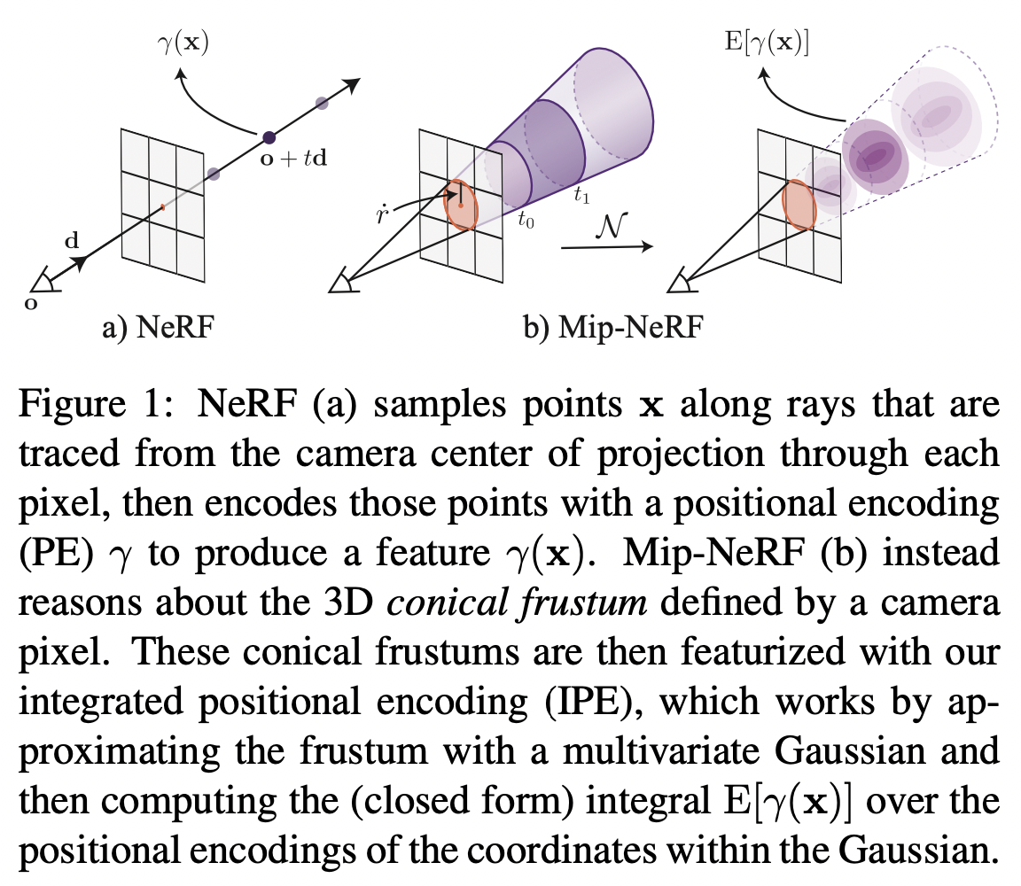
- Input: 3D Gaussian (It represents the region over which the radiance field should be integrated.)
- How to encode a 3D position and its surrounding Gaussian region?
- using integrated positional encoding (IPE): This is a generalization of NeRF’s ptositional encoding (PE) that allows a region of space to be compactly featurized, as opposed to a single point in space. (Space 라는 점으로 연속된 공간을 점 단위로 encoding 하는 것이 아닌, 각 공간을 단위로 압축적으로 encoding 한 feature를 통해 다루는 방법)
- Scale-aware Structure
- Problems of the NeRF (Point-sampling)
- sampling
- aliasing
2. Related Works
- Aliasing artifacts 를 해결하기 위한 방법
- Pre-filtering
- Supersampling

Aliasing artifact 1) Preliminary: NeRF
- NeRF는 Multilayer Perceptron(MLP)을 통해 하나의 이미지(scene)를 빛을 막거나 반사할 수 있는 입자(particle)로 이루어진 연속적 부피공간(a continuous volumetric field of particles)으로 모델링한다.
- 카메라의 각 픽셀을 렌더링 하는 방법:
- Ray (emitted from the camera's center of projection \(o\) along the direction \(d\) and it passes through the pixel): $$r(t) = o + td$$ * $t$ 는 거리를 의미한다.
- 샘플링 방법 (Sampling strategy)
- 카메라의 near, far 초점 거리에 수직인 면 $t_{n}$, $t_{f}$ 사이의 벡터를 결정하기 위해 사용한다.
used to determine a vector of sorted distances $t$ between the camera’s predefined near and far planes $t_{n}$ and $t_{f}$.
- 카메라의 near, far 초점 거리에 수직인 면 $t_{n}$, $t_{f}$ 사이의 벡터를 결정하기 위해 사용한다.
- $t_{k}$에 해당하는 거리를 Ray 위의 3D 위치($x$)로 변환한다.
Corresponding 3D position along the ray at the distance $t_{k} \in t$: $x = r(t_{k})$ - PE를 사용하여 각 위치를 변환:
Transform each position using a PE: $$\gamma (x)=\left[ \sin{(x)}, \cos{(x)}, ... , \sin{(2^{L-1} x)}, \cos{(2^{L-1} x)} \right]^T$$- NeRF 모델의 신뢰도는 PE 사용 여부에 따라 결정된다.
The fidelity of NeRF depends critically on the use of positional encoding. - L은 보간 커널 (interpolation kernel) 의 대역폭 (bandwidth) 을 결정한다.
$L$ determines the bandwidth of the interpolation kernel. - PE는 MLP가 이미지(scene)에 대해 interpolation 할 수 있도록 만들어준다.
PE allows the MLP parameterizing the scene to behave as an interpolation function. - 각 ray 위치에서의 PE:
The PE of each ray position: $$\gamma ( r{(t_{k})} )$$
- NeRF 모델의 신뢰도는 PE 사용 여부에 따라 결정된다.
- MLP의 입력값 (A MLP is parameterized by weights $\theta$, which outputs a density $\tau$ and an RGB color c):
$$\forall t_{k} \in t, \left[ {\tau}_{k}, c_{k} \right] = MLP(\gamma ( r{(t_{k})} ); \Theta)$$- The PE of each ray position ($\gamma ( r{(t_{k})} )$)
- View direction
- 구분구적법을 사용하여 볼륨 렌더링의 적분 연산을 근사한다.
Approximate the volume rendering integral using numerical quadrature: $$C(r; \Theta, t) = \sum_{k} T_{k} \left( 1-exp \left( -\tau_{k} \left( t_{k+1} - t_{k} \right) \right) \right) c_{k},$$ $$T_{k} = exp(- \sum_{k^{'} < k} \tau_{k^{'}} (t_{k^{'} + 1} - t_{k^{'}}))$$- $C(r; \Theta, t)$ is the final predicted color of the pixel.
- Hierarchical volume sampling: $$\min_{\Theta^{c}, \Theta^{f}} \sum_{r \in R} \left( \lVert C^{*}(r) - C(r;\Theta^{c}, t^{c}) \rVert^{2}_{2} + \lVert C^{*}(r) - C(r; \Theta^{f}, sort(t^{c} \cup t^{f}))\rVert^{2}_{2} \right) $$
- $C^{*}(r)$ is the observed pixel color taken from the input image.
3. Method
- Integrated Positional Encoding (IPE): a representation of the volume covered by each conical frustrum.
- The IPE allows the MLP to reason about the size and shape of each conical frustrum (instead of just its centroid).

The difference cause by using IPE (same position at different scales) 1) Cone Tracing
NeRF와 마찬가지로 MipNeRF 또한 한 픽셀씩 렌더링 된다. 따라서 이후에 나올 렌더링에 관한 설명은 하나의 픽셀을 단위로 한다.
- Cone: 카메라의 Projection 중심 ($o$) 에서 부터 해당 픽셀의 중심을 지나는 방향 ($d$) 으로 원뿔을 만든다.
- 꼭짓점의 위치: $o$
- 이미지 평면과 만나는 원뿔 단면(conical frustrums)의 반지름의 parameterization: $\dot{r} = o + d$
- $\dot{r}$ 을 world coordinate 에서 pixel의 너비로 지정한다.
- 두개의 $t$ 값 사이의 conical frustrum에 위치한 $x$의 집합을 수식으로 표현하면 다음과 같다 (Fig. 1의 $t_{0}, t_{1}$을 예로 들 때). $$F(x, o, d, \dot{r}, t_{0}, t_{1}) = \left\{ \left( t_{0} < \frac{d^{T} (x-o)}{\lVert d \rVert^{2}_{2}} < t_{1} \right) \wedge \left( \frac{d^{T} (x-o)}{\lVert d \rVert_{2} \lVert x-o \rVert_{2}} > \frac{1}{\sqrt{1 + {(\dot{r} / \lVert d \rVert_{2})}^{2}}} \right) \right\}$$
- 만약 $x$가 $(x, o, d, \dot{r}, t_{0}, t_{1})$로 정의된 conical frustrum 안에 위치해 있다면, $F(x, \cdot ) = 1$이다.
- (NeRF 학습에 매우 중요) Multivariate Gaussian: Conical frustrum 내부 volume을 표현하는 feature
- 다양한 방법이 있을 수 있지만, 가장 직관적이면서 효과적인 방법은 아래와 같이 Conical frustrum volume의 모든 coordinate에 대해 PE를 계산하는 것이다. $$\gamma^* (o, t, \dot{r}, t_{0}, t_{1}) = \frac{\int \gamma (x) F(x, o, d, \dot{r}, t_{0}, t_{1})dx}{\int F(x, o, d, \dot{r}, t_{0}, t_{1}) dx}$$
- 위의 식의 분자에 위치한 적분식은 closed problem 이 아니여서, 다변량 가우시안 (multivariate Gaussian)을 활용하여 근사하여 사용한다 (Integrated Positional Encoding (IPE)).
- $\mu_{t}, \sigma_{t}^{2}, \sigma_{r}^{2}$을 활용하여 Gaussian 구하기 (mid point: $t_{\mu} = (t_{0} + t_{1})/2$, half width (critical for numerical stability): $t_{\delta} = (t_{0} - t_{1})/2$)
- ray의 평균 거리: $\mu_{t} = t_{\mu} + \frac{2t_{\mu}t_{\delta}^{2}}{3t_{\mu}^{2} + t_{\delta}^{2}}$
- ray의 분산: $\sigma_{t}^{2} = \frac{t_{\delta}^{2}}{3} - \frac{4t_{\delta}^{4}(12t_{\mu}^{2} - t_{\delta}^{2})}{15(3t_{\mu}^{2} + t_{\delta}^{2})^{2}}$
- ray의 수직 분산 (variance perpendicular): $\sigma_{r}^{2} = \dot{r}^{2}\left( \frac{t_{\mu}^{2}}{4} + \frac{5t_{\delta}^{2}}{12} - \frac{4t_{\delta}^{4}}{15(3t_{\mu}^{2} + t_{\delta}^{2})} \right)$
- Multivariate Gaussian: Conical frustrum의 좌표계 상의 Gaussian을 world 좌표계로 변환 $$\mu = o + \mu_{t} d, \quad \sum=\sigma_{t}^{2}(dd^{T}) + \sigma_{r}^{2}\left( I - \frac{dd^{T}}{\lVert d \rVert_{2}^{2}} \right)$$
- $\mu_{t}, \sigma_{t}^{2}, \sigma_{r}^{2}$을 활용하여 Gaussian 구하기 (mid point: $t_{\mu} = (t_{0} + t_{1})/2$, half width (critical for numerical stability): $t_{\delta} = (t_{0} - t_{1})/2$)


(좌) Positional Encoding (PE), (우) Integrated Positional Encoding (IPE) 2) Integrated Positional Encoding (IPE)
- Positional Encoding (PE) 는 각 dimension 을 독립적으로 인코딩한다.
- Viewdirs는 PE로 인코딩 되고, Sample은 IPE로 인코딩 된다.
- Integrated Positional Encoding (IPE): the expectation of a positionally-encoded coordinate distributed according to the aforementioned Gaussian.
- Rewrite the PE as a Fourier feature: $$P=\begin{bmatrix} 1 & 0 & 0 & 2 & 0 & 0 & & 2^{L-1} & 0 & 0 \\ 0 & 1 & 0 & 0 & 2 & 0 & ... & 0 & 2^{L-1} & 0 \\ 0 & 0 & 1 & 0 & 0 & 2 & & 0 & 0 & 2^{L-1} \end{bmatrix}^{T} , \quad \gamma (x)=\begin{bmatrix} sin(Px) \\ cos(Px) \end{bmatrix}$$
- Lift the multivariate Gaussian: $$\mu_{\gamma} = P\mu ,\quad \sum_{\gamma} = P\sum P^{T}$$
- Expectations over lifted multivariate Gaussian $$\mathsf{E}_{x \sim \mathcal{N}(\mu, \sigma^{2})}[sin(x)] = sin(\mu) exp \left( -(1/2)\sigma^{2} \right)$$ $$\mathsf{E}_{x \sim \mathcal{N}(\mu, \sigma^{2})}[cos(x)] = cos(\mu) exp \left( - (1/2) \sigma^{2} \right)$$
- IPE with the diagonal of the covariance matrix: $$\begin{align} \gamma \left( \mu, \sum \right) &= \mathsf{E}_{x\sim \mathcal{N}(\mu_{\gamma}, \sum_{\gamma})} [\gamma (x)] \\ &= \begin{bmatrix} sin(\mu_{\gamma}) \circ exp(-(\frac{1}{2}) diag(\sum_{\gamma})) \\ cos(\mu_{\gamma}) \circ exp(-(\frac{1}{2}) diag(\sum_{\gamma})) \end{bmatrix} \end{align}$$ * 기호 $\circ$ 는 element-wise multiplication을 의미한다.
- $diag(\sum_{\gamma})$ 는 계산량이 매우 많다.
- IPE의 간격(interval)과 PE 주파수(frequency)의 주기(Period)에 따라 인코딩 결과가 달라진다 (즉, IPE의 간격에 대해 PE 의 주파수가 일정하면 보존하고, 주파수가 달라지면 제거한다).
- IPE방식은 point가 아니라 Gaussian regions를 사용하여 좌표기반의 neural network에 지역을 input으로 넣어줄 수 있다. 만약 더 넓은 지역을 본다면, higher frequency features는 자동으로 zero를 향해 줄어들어 network에게 lower-frequency inputs를 제공한다. 반대로 좁은 지역에서 이 features는 기존의 positional encoding과 비슷한 features 제공한다.
- 간격 (Interval) > 주기 (Period):
- PE: 하이퍼파라미터 L에 따라 일괄적으로 범위 내의 모든 주파수를 보존한다.
- IPE: 해당 주파수에서 인코딩 된 값들은 0으로 크기를 고정한다.
- 간격 < 주기:
- PE: 위와 동일
- IPE: 해당 주파수에서 인코딩 된 값을 그대로 사용한다.
더보기Positional Encoding 에 관해 현재까지 이해한 내용 정리: 1) x를 PE(x)로 푸리에 변환시 계수를 사용하지 않는 이유는 주파수 크기 비교가 아닌 주파수에 변화가 있는지를 확인하기 위해서 변환하기 때문이다. 2) 주파수 변화의 의미는 각 색마다 고유 주파수가 있을 때, 해당 위치가 색 A인 경우, A에 해당하는 주파수만 반사되어 유지되고 나머지 주파수들은 변화가 생기기 때문에 IPE에서 간격보다 주기가 작은 주파수들은 무시하는 이유는 해당 위치에 해당 주파수의 색은 없기 때문이라고 해석하기 때문이다.
The difference between PE and IPE (in 1D domain) 3) Architecture
- Mip-NeRF는 JaxNeRF 를 기반으로 구현되었다.
- 각 픽셀에 Ray 대신 원뿔(cone)이 캐스팅 된다는 점을 제외하고는 NeRF와 비슷하게 동작한다.
- $t_{k}$에 대해 $n+1$개의 값(IPE features)을 샘플링한다 (NeRF는 n개의 값 샘플링).
- Single Multiscale MLP 를 사용한다 (NeRF는 hierarchical MLP-coarse, fine-를 사용한다).
- Optimizatioin objective: $$\min_{\Theta} \sum_{r \in \mathcal{R}} (\lambda \begin{Vmatrix} C^{*} (r) - C(r; \Theta , t^{c} ) \end{Vmatrix}_{2}^{2} + \begin{Vmatrix} C^{*} (r) - C(r; \Theta , t^{f} ) \end{Vmatrix}^{2}_{2}$$
- Coarse Sample ($t_{c}$): Stratified Sampling 으로 샘플링
- Fine Sample ($t_{f}$): 수정된 alpha compositing weights ($w'$) 를 Inverse Transform Sampling 을 통해 샘플링 $$w^{'}_{k} = \frac{1}{2} \left( \max (w_{k-1}, w_{k}) + \max (w_{k}, w_{k+1}) \right) + \alpha$$ *2-tap max filter + 2-tap blur filter (원하는 특정 주파수를 거르기 위해... taps: DSP filter를 사용할 때 실제로 사용되는 샘플의 수)
4. Results
- 데이터셋
- 평가 (Evaluation)
- Blender Dataset (Same focal length and resolution)
- Multiscale Blender Dataset (Design to probe aliasing and scale-space reasoning)
- 평가 (Evaluation)


Blender Dataset 

Multiscale Blender Dataset - Metrics
- PSNR
- SSIM
- LPIPS
- the geometric mean of MSE, $\sqrt{1-SSIM}$, LPIPS
참조
