[논문리뷰] NeRFusion: Fusing Radiance Fields for Large-Scale Scene Reconstruction

 

CVPR 2022 (Oral) [Paper][Code]

Authors (University of California, San Diego, Adobe Research)

• Xiaoshuai Zhang
• Sai Bi
• Kalyan Sunkavalli
• Hao Su
• Zexiang Xu

 

Citation
@article{zhang2022nerfusion,
  author    = {Zhang, Xiaoshuai and Bi, Sai and Sunkavalli, Kalyan and Su, Hao and Xu, Zexiang},
  title     = {NeRFusion: Fusing Radiance Fields for Large-Scale Scene Reconstruction},
  journal   = {CVPR},
  year      = {2022},
}

---

0. Abstract

기존 모델의 문제점

• NeRF
  • MLP 크기 제한
  • 장면당 최적화(Per-scene optimization)가 필요하기 때문에 시간이 오래걸림
  • 큰 장면 (large-scale scenes) 을 렌더링하기 어려움
  • Small-scale scene, Object-centric scene
• Classical 3D Reconstruction Methods
  • 렌더링이 현실적이지 않다.

NeRFusion Proposals

• 효과적으로 대규모 이미지를 재구성하며 현실적인 렌더링이 가능하도록 NeRF 와 TSDF-based fusion 의 장점을 합치기.
  To achieve fast, large-scale scene- level radiance field reconstruction.
• Proposed novel RNN 을 사용하여 예측된 per-frame local radiance fields를 fusing 하여 global, sparse 한 장면을 22fps 속도로 실시간 렌더링 한다 (Global Volume).
• 대규모 실내 이미지 및 작은 크기의 장면에서 SOTA 를 달성하였다.

1. Introduction

Small-scale, Object-centric 한 장면이 아닌, 실내의 전면(full-size indoor scenes)을 렌더링 하기 위해 ScanNet scenes와 같은 large-scale 을 사용하였다. 또한, 대규모 장면을 빠르게 생성하기 위해 large sparse radiance fields를 점진적으로 reconstruct 하는 새로운 RNN 프레임워크를 제안한다.

NeRFusion 의 특징

• Generalizable
• Pre-trained across scenes
• Efficiently reconstructing large-scale (scalability) radiance fields via direct network inference 

NeRFusion은 재현된 Radiance fields를 모든 장면의 위치에 대해 3선형 보간(tri-linearly interpolated)된 voxel features로 이루어진 Sparse volume grid로 표현한다. 카메라 포즈와 함께 RGB 이미지 Sequence를 입력값으로 받아 classic TSDF 작동순서와 비슷하게 디자인된 파이프라인을 통과한다. Per-view geometry (depth) 에서 시작하여 per-view reconstruction을 모든 장면에 대해 fusing 하여 global sparse TSDF volume을 계산한다. NeRFusion은 기하학적 재구성(Geometric reconstruction)만 집중한 TSDF workflow와 달리 Novel RNN을 사용하여 sparse voxel을 구성한다.

Recurrent neural fusion module

• 순차적으로 여러 local fields를 모든 프레임에 대해 결합시킨다.
  Sequentially fuse multiple local fields across frames.
• 새롭게 추정된 local fields를 입력값으로 사용한다.
  Recurrently takes a newly estimated local field as input.
• 새로운 voxel을 추가되며 기존에 있던 voxel들을 업데이트 하는 방식으로 global radiance field로 장면을 재현할 수 있도록 순차적으로 voxel을 합치며 학습한다.
  Learns to incorporate the local voxels to progressively reconstruct a global radiance field modeling the entire scene, by adding new voxels and updating existing voxels.
• 전체 모델은 end-to-end 방식으로 학습된다. Radiance field 학습은 이미지 크기와 이미지 개수를 통제하지 않은 상태로 수행된다.
  Full model is trained from end to end, learning to reconstruct radiance fields with arbitrary scene scales from an arbitrary number of input images.

Training Datasets

• ScanNet Dataset
• DTU Dataset
• Google Scanned Object Dataset

2. Related Works

1) Multi-view Scene Reconstruction

기존 방법 (Previous methods to reconstruct geomery)

깊이 정보 (depth) 를 얻기 위해서 사용하는 방법은 1) multi-view stereo 2) depth sensor 가 있다. 최근에는 깊이를 측정하지 않고 학습을 통해 추정하는 방식을 사용한 Learning based multi-view stereo based on plane-swept cost volumes 연구도 등장했다. 측정한 깊이 값을 사용해 장면을 표현하는 방법의 종류는 아래의 두가지 종류가 있다.

1. Colored point clouds and utilizing point splatting to render images of the scene
2. Fuse multi-view depths and reconstruct surface meshes using techniques such as TSDF fusion or Poisson reconstruction

기존 방법의 문제점

: sensitive to potential inaccuracies in point clouds and meshes

• 원인: corrupted depth, especially when there are thin structures and textureless regions
• 결과: suffering from holes and blurry artifacts in the final renderings.

네트워크를 적용한 해결 방법과 문제점

• 제안된 방법: 2D CNN in screen-space to mitigate the potential errors in the geometry
• 문제점:
  • A per-scene optimization (long optimization time)
  • The screen-space neural networks produce temporally unstable results with flickering artifacts.
  • Only focus on geometry reconstruction.
  • Cannot produce realistic rendering.

Truncated signed distance function (TSDF) fusion techniques

 

2) Neural Radiance Fields

NeRF 적용 사례

• Relighting
• Scene editing
• Dynamic scene modeling

NeRF의 문제점

• Time-consuming (train MLP networks, specific for each scene from scratch, which can take hours and even days to optimize)
• Hard to scale up to large scene reconstruction (because of limited network capacity of MLPs).

해결 방법과 문제점

• NVSF
  • improves the scalability by building sparse voxel grids with per-voxel features.
  • 문제점: Time-consuming (per-scene optimization from scratch)
• PixelNeRF
  • uses 2D CNNs to extract image features on each sampled point of each ray
  • 문제점: 1) Object rendering with few images 2) trained specifically for each dataset
• IBRNet
  • enables rendering on any scene scales
  • 문제점: it leverages image features from neighboring views as input, varying across novel viewpoints, which often lead to blurry or flickering artifacts from sparse inputs.
• MVSNeRF
  • reconstructs 3D volumes
  • 문제점: it focuses on reconstructing a local volume from a fixed number of three nearby views.

3. Method

NeRFusion은 이미지를 프레임 단위로 순차적으로 받아 sequence를 direct network inference를 통해 sparse reconstruction으로 변환하는 점에서 장면당 최적화를 하는 방법들과 다르다. 

Scene 과 Frame의 차이는 무엇일까? (unofficial)

Scene은 object centric한 view로 동일한 origin pose와 서로 다른 direction을 가진 경우를 의미하고, Frame은 origin과 direction이 모두 다른 것을 의미하는 것으로 파악된다.

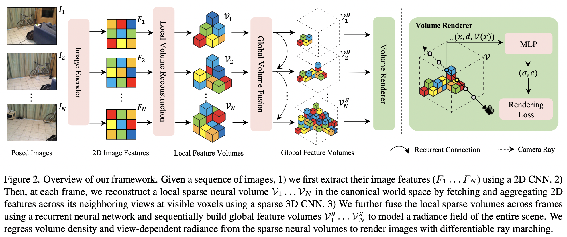
NeRFusion Pipeline

1. 지역적 프레임에 대한 local radiance field를 표현하는 밀도가 작은 볼륨 $\mathcal{V}_{t}$을 각 이미지 프레임에 대해 재현하기 위해 학습한다.
   Learns to reconstruct a sparse volume $\mathcal{V}_{t}$ per input image frame, expressing a local radiance field covered by local frames.
2. 재귀적인 융합 모듈은 각 프레임에 대한 볼륨($\mathcal{V}_{t}$)을 온라인으로 융합할 수 있도록 학습하는데, 이를 활용하여 점진적으로 전역적인 큰 규모의 영역($\mathcal{V}^{g}$)을 재현한다.
   Leverages a recurrent fusion module that learns to fuse the per-frame volumes $\mathcal{V}_{t}$ online, incrementally reconstructing the global large-scale field $\mathcal{V}^{g}$.
3. 전체 파이프라인을 기본 렌더링 loss를 사용하여 end-to-end 방식으로 학습시킨다.
   Train full pipeline from end-to-end with pure rendering losses.
4. 직접 네트워크 추론을 하여 고품질 radiance fields를 복원한다.
   Reconstruct high-quality radiance fields from direct network inference.

1) Sparse Volumes for Radiance Fields

NeRFusion은 radiance fields(output)을 $\mathcal{V}$(sparse neural volume)으로 모델링한다. $\mathcal{V}$는 서로 다른 특징을 가진 복셀들의 집합을 가지고있다. 복셀의 집합은 실제 장면을 대략적으로 포함하고 있다 (일부 포함안된 부분 있음). $$\sigma, c = R(x, d, \mathcal{V} (x))$$

• $\mathcal{V} (x)$: the tri-linearly interpolated feature at $x$
• $R$: the MLP

Pipeline

• 모든 시퀀스에 대해 희소볼륨은 프레임($t$) 마다 지역적 $\mathcal{V}_{t}$으로 재현된다.
  Sparse volumes are reconstructed locally as $\mathcal{V}_{t}$ per frame $t$ for the entire sequence.
• 모든 시퀀스에 대해 희소볼륨은 전역적 $\mathcal{V}_{g}$으로 재현된다.
  Sparse volumes are reconstructed globally as $\mathcal{V}_{g}$ for the entire sequence.
• MLP 네트워크 $R$은 트레이닝 과정에서 모든 볼륨이 공유한다.
  The MLP network $R$ is shared across all volumes in the training process.
• 정규좌표계에서 지역볼륨과 전역볼륨을 모델링한다.
  Model the local volumes and the global volume both in the canonical world space.

2) Reconstructing Local Volumes

• $K-1$개의 주변 이미지를 사용하여 더 정확하게 로컬볼륨($\mathcal{V}_{t}$)을 추론하여 이미지($I_{t}$)를 예측한다.
• 로컬볼륨($\mathcal{V}_{t}$)을 일반화 시키기 위해 정규좌표계에서 deep MVS 기법을 사용한다.
• 로컬볼륨($\mathcal{V}_{t}$)을 전역 볼륨($\mathcal{V}_{g}$)과 융합시킨다.

각 프레임($t$)의 local volume ($\mathcal{V}_{t}$)을 예측하기 위해서 이미지 $I_{t}$와 $K-1$개의 주변 이미지를 사용하는데, 다량의 주변 이미지를 사용하는 것은 이미지의 기하학적 의미를 더 정확하게 해석할 수 있게 도와준다. 
We propose a deep neural network to regress a local neural volume for each input frame $t$, using its image $I_{t}$ and $K-1$ images from neighboring views. usually, given a monocular video, these neighboring views correspond to temporal neighboring frames. Using multiple nearby images for per-frame reconstruction allows the network to leverage multi-view correspondence to recover better scene geometry, which a single image cannot provide. 

$\mathcal{V}_{t}$를 모든 장면에 대해 일반화 시키기 위해서 이 논문에서는 일반화 하여 적용할 수 있는 deep MVS 기법을 사용한다. 2D 이미지 특성을 추출하여 cost volume을 설정하고 $\mathcal{V}$를 cost volume으로 부터 산출해낸다. 하지만, frustrum volume을 시점(view's perspective)의 좌표에서 캐스팅한 MVSNeRF 및 MVS 기법을 사용한 다른 방법들과는 달리 NeRFusion은 정규좌표계에서 볼륨을 만들기 때문에 최종 결과물인 전역 볼륨($\mathcal{V}_{g}$)와 잘 호환되어 fusion 과정을 쉽게 수행할 수 있다.
To make the local reconstruction per frame well generalized across scenes, we leverage deep MVS techniques, which are known to be generalizable. We extract 2D image features, build a cost volume from the features, and regress a neural feature volume from the cost volume. However, unlike MVSNeRF and other MVS techniques that built frustrum volumes in view's perspective coordinate, we construct volumes in the canonical world coordinate frame to align it with the final global volume output $\mathcal{V}_{g}$, facilitating the following fusion process.

Image feature extraction

2D conv를 사용하여 각 이미지의 2D 이미지의 특성을 추출하였다. 이 네트워크는 입력으로 들어온 이미지($I_{t}$)를 2D 특성 맵($F_{t}$)로 맵핑시켜주는 역할을 하며 각 방향에서 바라본 장면을 인코딩한다.
We use a deep 2D convolutional neural network to extract 2D image features for each input image. This network maps the input image ($I_{t}$) into a 2D feature map ($F_{t}$), encoding the scene content from each view.

Local sparse volume

* sparse 하다는 의미가 모든 뷰에서도 보이지 않는 voxel들을 제거했기 때문이였다.

• Frustrm은 K개의 이웃한 뷰포인트를 포함하는데 어떠한 뷰에서도 보이지 않는 복셀들은 마스킹으로 제거한다.
• 마스킹 후, feature들을 unproject 시킨다.

정규좌표계상의 K개의 이웃한 뷰포인트를 포함하는 frustrum의 bounding box는 축에 정렬되어 있는데, 이 박스 안에 있는 voxel들은 서로 다른 뷰에서 봐야 볼 수 있는 경우도 있다. NeRFusion은 모든 뷰에서 보이지 않는 voxel들을 마스킹하여 제거하여 몇개의 voxel들만 남겨놓는다. 지역적 이미지 인코딩을 위해 투형했던 이미지 특성들을 다시 투영해제(unproject) 시킨다.
We consider the bounding box that covers the frustums of all K neighboring viewpoints in the world coordinate frame, containing of a set of voxels in the canonical space. The bounding volume is axis-aligned with the world frame; each voxel inside it can be visible to a different number of neighboring views. We mask out all the voxels invisible to all view, leading to a sparse set of voxels in the bounding box. We then unproject the image features into this volume for our local reconstruction.

3D feature volume

• 이웃한 뷰포인트 feature map($F_{i}$)의 3D feature 볼륨($\mathcal{U}_{i}$)을 만든다.
• $\upsilon$을 중심으로 한 복셀을 통해 뷰($i$)의 3D 볼륨($\mathcal{U}_{i}(\upsilon)$)을 추정한다. $$\mathcal{U}_{i}(\upsilon) = \left[ F_{i}(u_{i}), G(d_{i}) \right]$$

각각의 이웃한 뷰포인트 $i$와 이웃한 뷰포인트의 Feature map($F_{i}$)마다 3D 특성 볼륨($\mathcal{U}_{i}$)를 만든다. 특히, 각각의 $\upsilon$을 중심으로 한 관찰 가능한 복셀은 프레임 $t$에서 이웃한 뷰포인트를 2D 사영한 후 이미지 특성을 추출한다. 단순 이미지 특성 뿐만 아니라 각각의 뷰포인트의 $\upsilon$에서 해당 뷰 방향 $d_{i}$을 활용하고 MLP($G$)를 통해 추출한 추가 특성을 계산하여 활용한다. 각 뷰($i$)의 3D 볼륨($\mathcal{U}_{i}$)는 다음과 같이 나타낸다.
For each neighboring viewpoint $i$ and its feature map $F_{i}$, we build a 3D feature volume $\mathcal{U}_{i}$. In particular, for each visible voxel centered at $\upsilon$, we fetch the 2D image feature at its 2D projection from each neighboring view at frame $t$. In addition to pure image features, we leverage the corresponding viewing direction $d_{i}$ at $\upsilon$ from each viewpoint and compute additional features using an MLP $G$. The per-view 3D volume $\mathcal{U}_{i}$ is expressed by
$$\mathcal{U}_{i}(\upsilon) = \left[ F_{i}(u_{i}), G(d_{i}) \right]$$

$\mathcal{U}_{i}(\upsilon)$는 $\upsilon$을 중심으로 한 복셀의 특성을 나타낸다. $u_{i}$는 뷰 $i$에서 $u_{i}$의 중심을 2D 사영한 것을 나타낸다. $[·, ·]$는 특성을 합친것을 의미한다. reconstruction 과정에서 입력된 뷰의 방향에 대한 정보를 추가적으로 활용하여 인코딩한다; viewdirs는 앞으로 설명할 퓨전 모듈이 모든 프레임에 대해 뷰의 영향을 받는다는 사실을 잘 설명해준다.
where $\mathcal{U}_{i}(\upsilon)$ is the feature at a voxel centered at $\upsilon$, $u_{i}$ is the center’s 2D projection in view $i$, $[·, ·]$ represents feature concatenation. Note that, we encode the additional information of input viewing directions in the reconstruction process; this crucial information makes our following fusion module effectively account for the view-dependent effects captured across frames.

Neural reconstruction

• 로컬볼륨($\mathcal{V}_{t}$)를 추정하기 위해 이웃한 뷰포인트의 특징($\mathcal{U}_{i}$)을 이용하여 합친다.
• 딥러닝 네트워크 $J$를 사용하여 각 복셀의 평균과 분산을 계산한다. $$\mathcal{V}_{t} = J\left( \left[ Mean_{i \in \mathcal{N}_{t}} \mathcal{U}_{i}, \quad Var_{i \in \mathcal{N}_{t}} \mathcal{U}_{i} \right] \right)$$
• 퓨전 모델을 사용하여 $\mathcal{V}_{t}$를 $\mathcal{V}_{g}$로 융합시킨다.

다음으로는, 프레임($t$)에서 Local volume($V_{t}$)를 추정하기 위해 다수의 이웃한 뷰포인트의 특징들을 합쳐준다. NeRFusion은 $\mathcal{U}_{i}$에서 이웃한 뷰포인트에서 계산한 각 복셀 feature의 평균과 분산을 활용한다; 이러한 과정은 MVS를 사용하는 기법에서 cost volume을 만드는데 주로 사용되며 평균값은 각 뷰의 appearance를 융합할 수 있고, 분산은 기하학 추론을 위한 풍부한 정보를 제공해준다. 이 두가지 작업은 입력값의 개수와 순서와 관계없이 일정하다; NeRFusion의 경우, 이러한 작업이 각 복셀이 서로 다른 개수의 관찰가능한 뷰포인트를 처리할 수 있도록 만들어준다. 딥러닝 네트워크 $J$를 사용하여 각 복셀의 평균과 분산을 계산하여 각 뷰를 reconstruction 하는 과정은 다음과 같다.
We then aggregate the features across multiple neighboring viewpoints to regress a local volume Vt at frame t, expressing a local radiance field. We propose to leverage the mean and variance of the per-voxel features in $\mathcal{U}_{i}$ computed across neighboring viewpoints; such operations have been widely used in building cost volumes in MVS-based techniques, where the mean can fuse per-view appearance information and the variance provides rich correspondence cues for geometry reasoning. These two operation are also invariant to the number/order of input; in our case, this naturally handles voxels that have different numbers of visible viewpoints. We use a deep neural network $J$ to process the mean and variance features per voxel to regress the per-view reconstruction by
$$\mathcal{V}_{t} = J\left( \left[ Mean_{i \in \mathcal{N}_{t}} \mathcal{U}_{i}, \quad Var_{i \in \mathcal{N}_{t}} \mathcal{U}_{i} \right] \right)$$

$\mathcal{N}_{t}$는 프레임($t$)에서 사용된 모든 이웃한 뷰포인트($K$개)를 나타낸다; 평균과 분산은 요소단위로 연산된 값을 의미한다.
Here $\mathcal{N}_{t}$ represents all $K$ neighboring viewpoints used at frame t; Mean and Var represent element-wise average and variance operation, respectively.

필수적으로, NeRFusion은 이웃한 뷰들의 feature로부터 local radiance field를 추론한다. 이 과정은 MVSNeRF와 유사하다. 하지만, local reconstruction과 small-baseline 렌더링을 위한 perspective frustrum volume 만을 고려하는 MVSNeRF와는 달리, local volume을 전역의 large-scale reconstruction과 렌더링하는 데 활용한다. NeRFusion은 정규 공간에서 볼륨을 직접 계산하고 자연적으로 프레임당 복셀 입력값을 퓨전 모델에 제공한다.
Essentially, we regress the local radiance field from the features across neighboring views. This is similar to MVS- NeRF. However, unlike MVSNeRF that considers only local reconstruction and builds perspective frustrum volumes for small-baseline rendering, we leverage these local volumes for global large-scale reconstruction and rendering. We build volumes directly in canonical space, naturally providing per-frame voxel inputs for our fusion module.

3) Fusing Volumes for Global Reconstruction

Gated Recurrent Unit (GRU) fusion step

장면 구현을 일정하고, 효율적이고, 확장 가능하게 하기 위해서 NeRFusion은 전역적 볼륨 합성 네트워크를 사용한다. 이 네트워크는 점진적으로 각 프레임의 지역적 볼륨 특성($\left\{ \mathcal{V}_{t} \right\}$)을 전역적 볼륨($\mathcal{V}_{g}$)으로 합성시킨다.
In order to create a consistent, efficient, and extensible scene reconstruction, we propose to use a global neural volume fusion network to incrementally fuse local feature volumes $\left\{ \mathcal{V}_{t} \right\}$ per frame into a global volume $\mathcal{V}_{g}$.

Fusion

• GRU(Gated Recurrent Unit)는 합성모듈이다.
• 로컬볼륨($\mathcal{V}_{t}$)을 구현하고, 이전 프레임을 재귀적으로 입력받아 글로벌볼륨($\mathcal{V}^{g}_{t-1}$)을 구성한다.
  $$z_{t} = M_{z} \left( \left[ \mathcal{V}^{g}_{t-1} , \mathcal{V}_{t} \right] \right)$$$$r_{t} = M_{r} \left( \left[ \mathcal{V}^{g}_{t-1} , \mathcal{V}_{t} \right] \right)$$$${\overset{\sim}{\mathcal{V}}}_{t}^{g} = M_{t} \left( \left[ r_{t} * \mathcal{V}^{g}_{t-1} , \mathcal{V}_{t} \right] \right)$$$$\mathcal{V}_{t}^{g} = (1 - z_{t} ) * \mathcal{V}^{g}_{t-1} + z_{t} * {\overset{\sim}{\mathcal{V}}}_{t}^{g} $$
• $M_{t}$는 tanh를 사용하여 전체 모델이 순차적으로 global reconstruction ($\mathcal{V}_{t}^{g}$)를 매 입력 프레임마다 업데이트 할 수 있도록 한다(GRU의 hidden state 참조).
• GRU는 업데이트게이트($z_{t}$)와 재설정게이트($r_{t}$)는 $\mathcal{V}^{g}_{t-1}$와 $\mathcal{V}_{t}$를 사용하여 $\mathcal{V}^{g}_{t}$를 업데이트한다.
• NeRFusion의 볼륨은 neural radiance fields를 학습한다.

각 프레임($t$)에서 지역적이고 희소한 볼륨($\mathcal{V}$)을 재현하고, 이전 프레임을 반복적(recurrent)으로 입력으로 받아 전역적 재현($\mathcal{V}^{g}_{t-1}$)을 한다. GRUs (Gated Recurrent Unit)을 희소 3D CNN과 함께 사용하여 합성 모듈을 구성하며 네트워크가 반복적으로(recurrently) 각 프레임의 지역적 재현과 함께 고품질의 전역 복사 영역(global radiance field)을 학습한다. 이러한 과정은 다음과 같다.
At each frame $t$, we consider its local sparse volume reconstruction V and the global reconstruction $\mathcal{V}^{g}_{t-1}$ from the previous frame as recurrent input. We leverage GRUs (Gated Recurrent Unit) with sparse 3D CNNs in our fusion module, allowing our network to learn to recurrently fuse the per-frame local reconstruction and output high-quality global radiance fields. This is expressed by 
$$z_{t} = M_{z} \left( \left[ \mathcal{V}^{g}_{t-1} , \mathcal{V}_{t} \right] \right)$$$$r_{t} = M_{r} \left( \left[ \mathcal{V}^{g}_{t-1} , \mathcal{V}_{t} \right] \right)$$$${\overset{\sim}{\mathcal{V}}}_{t}^{g} = M_{t} \left( \left[ r_{t} * \mathcal{V}^{g}_{t-1} , \mathcal{V}_{t} \right] \right)$$$$\mathcal{V}_{t}^{g} = (1 - z_{t} ) * \mathcal{V}^{g}_{t-1} + z_{t} * {\overset{\sim}{\mathcal{V}}}_{t}^{g} $$

∗ 는 요소별 곱하기를 의미한다. $z_{t}$와 $r_{t}$는 업데이트 게이트(update gate)와 재설정 게이트(reset gate)이고, $M_{z}, M_{r}, M_{t}$는 모두 딥러닝 네트워크로 희소 3D 컨볼루션 레이어로 구성되어 있다. 표준 GRU, $M_{z}, M_{r}$은 마지막에 시그모이드 활성함수를 통과하도록 디자인 되어 있고, $M_{t}$는 tanh를 사용하여 전체 모델이 순차적으로 global reconstruction ($\mathcal{V}_{t}^{g}$)를 매 입력 프레임마다 업데이트 할 수 있도록 한다(GRU의 hidden state 참조). 이 과정에서 NeRFusion은 네트워크를 지역 볼륨($\mathcal{V}_{t}$)으로 덮여있는 복셀에 적용한다; 이 때 다른 모든 전역 볼륨의 복셀들은 업데이트 되지 않는다. GRU 합성 과정은 Fig3에 다이어그램으로 표현되어 있다.
where ∗ is the element-wise multiplication, $z_{t}$ and $r_{t}$ are the update gate and the reset gate, $M_{z}, M_{r}$ and $M_{t}$ all deep neural networks with sparse 3D convolution layers. As in standard GRU, $M_{z}$ and $M_{r}$ are designed with sigmoid activation in the end, while $M_{t}$ uses tanh, allowing for the entire model sequentially updating the global reconstruction $\mathcal{V}_{t}^{g}$ (seen as the hidden state in a GRU) for every input frame. In this process, we only apply the networks on the voxels covered by the local volume $\mathcal{V}_{t}$; all other voxels in the global volume are kept unchanged. A 2D illustration of this GRU fusion process is shown in Fig. 3.

직관적으로 GRU의 업데이트게이트(z_{t})와 재설정게이트(r_{t})는 어느정도의 정보를 이전 프레임의 전역볼륨($\mathcal{V}^{g}_{t-1}$)과 현재 프레임의 지역볼륨($\mathcal{V}_{t}$)에서 가져와서 새로운 전역볼륨특성으로 업데이트 해야하는지 결정한다. 이러한 방식은 모듈이 상황에 맞춰 표현을 일정하게 유지하면서도 구멍을 메우거나 특성을 정제하는 방향으로 전체장면재현을 개선할 수 있도록 한다. 이러한 합성과정은 기하학적 재현에만 초점을 맞춘 이전의 3D 재현 파이프라인과 유사한데, NeRFusion은 볼륨이 볼륨 렌더링을 위한 neural radiance fields를 학습하도록 하여 사실적인 장면 합성을 할 수 있도록 한다.
Intuitively, the update gate zt and reset gate rt in the GRU determine how much information from the previous global volume Vg as well as how much information from t−1 the current local volume Vt should be incorporated into the new global features. In this way, our module can adaptively improve the global scene reconstruction by filling up holes and refining features while keeping the representation consistent. This fusion process is similar to previous 3D reconstruction pipelines that focus on geometry reconstruction; in contrast, we instead reconstruct neural feature volumes to represent neural radiance fields for volume rendering, leading to photo-realistic novel view synthesis.

Voxel pruning

• 프루닝을 통해 렌더링 과정을 효율적으로 만든다.
• 모든 프레임에서 $\mathcal{V}_{t}^{g}$를 구성할 때 불필요한 복셀들을 제거한다. $$\min_{i=1...k} exp (-\sigma (\upsilon_{i} )) > \gamma , \upsilon_{i} \in V$$

메모리와 렌더링 효율을 극대화시키기 위해 NeRFusion은 매 프레임마다 상황에 맞춰서 전역볼륨재현($V_{t}^{g}$) 과정에서 모든 장면에서 렌더링이 필요하지 않은 불필요한 복셀들을 제거하여 프루닝한다. 당연히 radiance field로부터 추정된 각 복셀의 볼륨의 밀도를 활용하여 장면의 지오메트리를 모델링한다. 특히, NeRFusion은 복셀($\mathcal{V}$)를 다음과 같을 때 프루닝한다.

To maximize the memory and rendering efficiency, we adaptively prune the global volume reconstruction Vtg for every frame by removing the non-essential voxels that do not have any scene content inside. We naturally leverage the volume density in each voxel regressed by our radiance field, which models the scene geometry. In particular, we prune voxels $\mathcal{V}$ if:
$$\min_{i=1...k} exp (-\sigma (\upsilon_{i} )) > \gamma , \upsilon_{i} \in V$$

$\left\{ \upsilon_{i} \right\}^{k}_{i=1}$가 복셀($\mathcal{V}$)이 $k$개의 균일하게 샘플링된 포인트를 가지고 있을 때, $\sigma{\upsilon_{i}}$가 $\upsilon_{i}$ 위치에서 예측된 밀도를 의미한다. $\gamma$는 프루닝 임계값을 의미한다. 이렇게 함으로써 NeRFusion은 전역볼륨의 밀도를 더욱 희박하게 만들 수 있고, 장면을 재현하고 렌더링하는 과정을 더욱 효율적으로 만들 수 있다.
where $\left\{ \upsilon_{i} \right\}^{k}_{i=1}$ are k uniformly sampled points inside the voxel V , σ(vi) is the predicted density at location vi, and γ is a pruning threshold. This pruning step is performed in both later training phase and inference phase once we get a global feature volume Vtg . By doing so, we make our global volume sparser, leading to more efficient reconstruction and rendering.

4) Training and Optimization

일단 radiance field가 만들어지면 NeRFusion는 다른 NeRF 모델들과 같이 회귀된 볼륨밀도와 뷰를 기반으로 한 radiance 를 사한 미분가능한 ray marching으로 최종 렌더링 된다. NeRFusion의 파이프라인은 정답 이미지를 통해 supervised learning으로 학습하고, 추가 기하학 정보를 통한 supervision은 사용하지 않는다. 

Once a radiance field (that is represented by a sparse neu- ral volume as described in Sec. 3.1) is reconstructed, our final rendering is achieved via differentiable ray marching using the regressed volume density and view-dependent radiance at any sampled ray points, as is done in NeRF and any other radiance field methods. In this work, our full pipeline is trained, completely depending on the rendering supervision with the ground truth images, without any extra geometry supervision.

특히, 로컬 렌더링 네트워크와 radiance field 디코더($R$)을 다음의 목적함수를 통해 훈련시킨다.
In particular, we first train our local reconstruction network and the radiance field decoder (R) with a loss
$$\mathcal{L}_{local} = \begin{Vmatrix} C_{t} - \overset{^}{C} \end{Vmatrix}^{2}_{2}$$

$\overset{^}{C}$은 정답 픽셀의 색을 의미하고, $C_{t}$는 로컬 볼륨 $\mathcal{V}_{t}$를 사용하여 렌더링된 픽셀의 색을 의미한다. 이미 네트워크가 지엽적으로 현실적인 이미지를 렌더링할 수 있지만, 더욱 리즈너블한 로컬볼륨을 예측하도록 학습한다; 또한, radiance field 디코더 MLP를 리즈너블한 상태로 초기화하여 로컬과 글로벌 볼륨에 공유한다. 이러한 프리트레이닝은 로컬 렌더링 모듈이 의미있는 볼륨 특징들을 퓨전 모듈이 end-to-end 훈련에 사용할 수 있도록 돕는다. 그 후, 전체 파이프라인인 로컬 렌더링 네트워크, 융합 네트워크, radiance field 디코더 네트워크를 rendering loss를 사용하여 end-to-end로 학습시킨다.
where Cˆ is the ground truth pixel color and Ct represents the rendered pixel color using the local volume Vt reconstructed at frame t. This makes the network learn to predict reasonable local neural volumes, which are already renderable and able to produce realistic images locally; it also initializes the radiance field decoder MLP to a reasonable state, which is later shared across local and global volumes. This pre-training allows the local reconstruction module to provide meaningful volume features for the fusion module to utilize in the end-to-end training, effectively facilitating the fusion task. We then train our full pipeline with the local reconstruction network, fusion network, and the ra- diance field decoder network all together from end to end, using a rendering loss.
$$\mathcal{L}_{fuse} = \sum_{t} \begin{Vmatrix} C_{t} - \overset{^}{C} \end{Vmatrix}^{2}_{2} + \begin{Vmatrix} C_{t}^{g} - \overset{^}{C} \end{Vmatrix}^{2}_{2}$$

$C_{t}$는 로컬 렌더링 $\mathcal{V}_{t}$를 사용해 렌더링한 픽셀의 색이고 $C_{t}^{g}$는 글로벌 볼륨($\mathcal{V}_{t}^{g}$)를 프레임 $t$에 대해 융합한 후 렌더링 한 색을 의미한다. 기본적으로, NeRFusion은 글로벌과 로컬 볼륨의 모든 중간단계에서 값을 가져와서 이미지를 렌더링한다. 그리고, 정답 이미지로 supervise한다. 그래서 퓨전 모듈은 리즈너블하게 로컬 볼륨을 다양한 수의 입력 프레임으로 부터 학습한다.
where Ct is the pixel color rendered from the local reconstruction Vt (as is in Eqn. 9) and Ctg is the color rendered from the global volume Vtg after fusing frame t. Basically, we take every intermediate global and local volume (Vt and Vtg) at every frame to render novel view images and supervise them with the ground truth. The fusion module thus reasonably learns to fuse local volumes from an arbitrary number of input frames.

훈련이 끝난 후, 네트워크는 고품질의 radiance field를 네트워크 추론을 직접 사용하여 현실적인 렌더링 이미지를 생산해낼 수 있다. 게다가, radiance field를 희소볼륨으로 복원하면 렌더링 품질을 높이기 위해 장면당 최적화를 하기 더 쉬워진다.
After trained, our full network is able to output a high-quality radiance field from direct network inference and produce realistic rendering results (as shown in Fig. 1). In addition, the reconstructed radiance field as a sparse neural volume can also be easily optimized (fine-tuned) per scene further to boost the rendering quality.

Fine-tuning

 

추정된 radiance field를 파인튜닝하기 위해서 NeRFusion은 복셀마다 네트워크 희소볼륨 $\mathcal{V}_{g}$ 복원하기 위한 feature들을 최적화하고, 포착된 이미지로 MLP 디코더의 각 장면을 최적화 한다. 처음 이미지 복원 결과가 이미 좋기 때문에, 짧은 최적화 시간(25k 반복횟수 이하)인 1시간 이하로도 매우 고품질의 렌더링이 가능하다. 이는 NeRF와 장면당 최적화를 하는 다른 방법들에 비해 매우 적은 최적화 시간이다.
To fine-tune the estimated radiance field, we optimize the per-voxel neural features in the sparse volume reconstruction Vg and the MLP decoder per scene with the captured images, leading to better rendering results. Since our initial reconstruction is already very good, a short period of optimization with less than 25k iterations can usually lead to very high quality, which takes less than 1 hour. This is substantially less optimization time than NeRF and other pure per-scene optimization methods.

매 장면의 최적화 단계에서 NSVF와 같이 NeRFusion은 coarse-to-fine 복원 과정을 거친다. 기본적으로, 매 10K 최적화 반복횟수 이후에 불필요한 복셀들을 프루닝하고 모든 복셀을 8개의 작은 복셀들로 나눈다. 이러한 프루닝과 분해 단계는 점진적으로 공간 해상도를 높이고, 최종 렌더링 퀄리티를 개선한다.
In this per-scene optimization stage, we also do a coarse-to-fine reconstruction, similar to NSVF. Basically, after every 10k optimization iterations, we further prune unnecessary voxels (using Eqn. 8) and also subdivide each voxel into 8 sub voxels. This prune and subdivision step progressively increases the spatial resolution of the neural volume, further improving our final rendering quality.

4. Implementation Details

Training datasets

Large scale indoor scene

• ScanNet: randomly sampled 100 scenes

Small Objects

• DTU: adopt the training split from PixelNeRF, which includes 88 training scenes.
• Google Scanned Objects: 1,023 models generated by Ibrnet

Training details

Datasets

• Object-centric datasets: sample 16 views for each scene
• ScanNet:
  • sample 2% − 5% of the full sequence as key frames
  • All other frames are used for supervision.
  • use K = 3 neighboring views for each input frame, for local volume reconstruction.
  • 3 neighboring key frames temporally.
• Other datasets:
  • select the 3 spatially closest viewpoints, in terms of both viewing location and direction.

Other Details

• The sparse volumes and networks are implemented with torchsparse

5. Results

 

Baselines

• NeRF
• NVSF
• NerfingMVS
• PixelNeRF
• IBR-Net
• MVSNeRF

Large-scale scenes in ScanNet

 

Showing significantly better results than IBRNet

Showing high visual quality on large-scale scenes

 

NeRF synthetic

DTU

 

6. Limitations

NeRFusion의 접근법은 큰 규모의 실내 장면을 위주로 다루고 있지만, 다양한 깊이의 물체를 다루는 장면에 대해서는 좋은 성능을 내지 않을 수 있습니다. 실외 장면들은 object의 크기가 제한되어 있지 않을 때가 많기 때문에 NeRFusion의 접근 방식이 올바르지 않을 수 있습니다. NeRFusion은 모든 장면에 대해 'Neural sparse voxel fields' 논문과 마찬가지로 동일한 크기의 복셀을 바탕으로 radiance field를 추정하고 있기 때문에, 이러한 규격화된 복셀이 정규좌표계가 아니거나 dynamic한 depth와 크기를 가진 object를 가진 장면인 경우 (NeRF++와 마찬가지로)에도 잘 적용될 수 있도록 연구가 필요합니다. NeRFusion은 여러개의 뷰에서 대응시키는 방식을 사용하였기 때문에 매우 극단적인 카메라 위치와 오브젝트간의 (거리차이로 인해 발생하는)시차가 있는 경우 잘 작동하지 않을 수 있습니다. 이러한 문제는 모든 MVS를 기반으로 하는 기법들에서 공통으로 발생하는 문제입니다. 현재 파이프라인 상에서는 NeRFusion은 입력된 프레임을 균일하게 샘플링하고 있으며, ScanNet의 카메라 움직임이 이미 충분히 해석되어있기 때문에 추가 perturbation을 하고있지 않습니다. 하지만, 신중하게 뷰를 선택하는 기법을 사용한다면, 다양한 카메라 모션을 가진 장면에 대해서도 학습을 할 수 있습니다.
Our approach currently focuses on handling large-scale indoor scenes, but might not be efficient on handling scenes that have foreground objects with distant background, which might appear in unbounded outdoor scenes. This is because we consider a uniform grid for the entire scene, similar to 'Neural sparse voxel fields'. This can be potentially addressed in the future by doing per-view reconstruction in disparity space or applying spherical coordinates for regions at long distances (similar to NeRF++). Our method relies on multi-view correspondence; hence, extreme camera poses without enough parallax could lead to problems, which cannot be addressed by any MVS-based techniques. For our current pipeline, we simply sample input frames uniformly, because the camera motion in ScanNet has enough translation. However, a more careful input view selection technique that accounts for relative camera poses may be necessary in practice to address various types of camera motions.

7. Conclusion